Special Topics in Strategy Design

PDF Version: P123 Strategy Design Topic 7 – Special – (i) Growth and (ii) Valuation Ratios Based on Q vs TTM

The following topics were inspired by an e-mail inquiry I received after completion of the main part of the course. It’s just as well this content comes in the context of post-graduate material. I think it would have been much more cumbersome to present were I unable to assume a certain foundation is already in place.

The topics to be discussed here are (i) Growth, and (ii) Valuation using Q metrics.

Growth

It was called to my attention that the main part of the seminar did not cover the “Growth” approach to investing. That will be rectified now.

In one sense, I did cover growth. The Dividend Discount Model (DDM) and all its variants uses growth as a critical input. The basic form of the model is D/(R-G). This, and each of the other variations that was discussed, puts G into the denominator as a negative number, which means that as G rises, so to does P all else being equal.

That was easy. The hard part if figuring out how, exactly, to incorporate a G factor into our models. We can’t literally plug any number into a DDM formula because DDM presumes we’re dealing with an infinite growth rate. The infinity angle forces us to plug in a very low G figure (theoretically reflecting an extremely mature company as one must be if it is to be around for infinity), and we need this lest we plug in a G in excess of R, something that would cause the model to produce a negative P.

Also, we don’t want G to be zero. In that case, stocks would be hard pressed to attract any investment at all relative to less risky-fixed income. So growth isn’t merely relevant to equity investing. It is the essence of equity investing!

But, as discussed, To apply DDM in the real world, we need lots of spit and chewing gum; creative approximations or proxies to stand in for G, and for R as well.

So yes, by discussing proxies for growth such as ROE (the capacity to grow) and sentiment, I have covered growth.

Then again, I did not cover growth the way many expect. What about all those growth-rate factors that are built into Portfolio123, not to mention the countless others you can create using your own formulas?

We start with the notion that all those numbers represent the past. Historic rates of growth mean nothing to us; absolutely positively nothing. But we have to have some sort of growth expectation. Can we not use historic growth rates as a proxy for future expectations based upon the idea that change is gradual, or evolutionary rather than revolutionary. Sure we’ll miss the mark here snd there as some companies quickly change course. But if we’re reasonably diversified, we should be able to control this form of “company-specific risk. So let’s bring historic growth rates into our model with full awareness of the relevant risks.

That’s OK, isn’t it? Yes . . . sort of. We can do it. But it may not be as simple as some suggest. Let’s walk through it.

Sales Growth

We know that ultimately, investors are concerned with earnings, cash flows and dividends. But aberrations aside (divestitures, recessions, etc.)  none of that is possible without Sales. And relative to other metrics, Sales has the advantage of being least subject to non-core accounting “stuff.” So sales growth can be, and many could argue should be a vital component of our strategies.

Table 1 summarizes a set of best-worst backtests conducted on the PRussell3000 Universe assuming 4-week rebalancing and running from 1/2/99through 6/16/16. 

I looked at four SalesItems:

• Sales%ChgPQ
• Sales%ChgPYQ
• Sales%ChgTTM
• Sales5YCGr%

Each of these was tested using best-worst portfolios constructed on the basis of the following screening rules:

• SalesItem != NA
• FRank(“SalesItem,”) > Best

 

• SalesItem != NA
• FRank(“SalesItem,”) < Worst

 

I used three sets of Best-Worst thresholds

• Simple
  • Best defined as >50
  • Worst defined as < 50
• Mainstream
  • Best defined as >75
  • Worst defined as < 25
• Aggressive
  • Best defined as >95
  • Worst defined as < 5

 If our theory that Sales growth is a legitimate investment factor is correct, we should generally expect a positive correlation between the growth rate we chose and the subsequent 4-week performance of the stock. The one-on-one matchup between items (or their ranks) may or may not be capable of giving us a highly positive correlation, but at the very least, the 95-5 dichotomy should be more productive than the 75-25  dichotomy which should, in turn, be better than the 50-50 split. Let’s see that illustrated in Table 1.

Table 1

 

Yuk, phooey!

That’s a hot mess! Actually, it’s much worse than a hot mess but I’d like to keep this printable. (Also, the table looks incomplete: Why didn’t I repeat the PQ experiments all the way through? That, actually, is the least of our concerns. I’ll come back to it laster.) 

Logically, the market has to care about sales growth. Perhaps this is so erratic as to make historical data completely useless. Or, perhaps, the market is so irrational as to not realize the deep connection between Sales and EPS.

EPS Growth

Let’s repeat the experiment only this time, we’ll use EPS growth items instead of items relating to Sales growth. Table 2 summarizes the results and should show another hot mess. No, actually, it should look worse considering how often EPS figures get distorted by aberrant accounting events.

Here it is.

Table 2

 

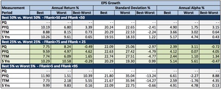
Oops again.

This was supposed to be worse than Sales items but it isn’t. Arguably, we see factors that might be useful. Skipping PQ again for the moment, we see that EPS growth makes a difference and that the market is most interested in whist happened most recently, the PYQ interval. Moreover, the TTM and 5-year figures are at least pointing in the right direction.

So we’ve got it. We know we can use EPS%ChgPYQ as a proxy for the G in the DDM, or in less academic terms, we can define growth in terms of EPS%ChgPYQ.

Not so fast.

Let’s not rush to lock in on a decent set of test results, even though they seem explainable. Is the explanation a good one?

Let’s go back to why we look at growth. We’re concerned about growth in the future. Remember, too, the DDM is an infinite series. Realistically, we know we aren’t going to model for an infinity holding period. But common sense tells us we need to be thinking in terms of at least some measure of sustainability. It’s not urgent that we put a number on this. We just have to think in terms of sustainable, normal, recurring, etc. Whatever that means, most of us would probably wonder if the myopic approach that relies on the latest PYQ figure is really the best way to represent it.

Maybe PYQ really is best. Wall Street is famous for being apathetic to the long term. But we can’t ignore the fact that EPS is a lesser proxy than Sales, which is not as prone to accounting oddities. If the PYQ figure really was a useful proxy for growth, then our Sales growth tests would not look so rotten. We might justify learning toward EPS if we want to argue stocks are being credited with margin improvement. But if that was what is happening, sales would be decent and EPS would be better. Yet we see dismal extremely sub-decent results for sales.

Table 2 is telling us something. But it’s hard to argue that its telling us EPS%ChgPYQ is the way to go if we’re interested in growth. I’ll give you the spoiler: It’s telling us something about noise and momentum. It can and should be used if that’s what you’re looking for, and on this basis, EPS%ChgPYQ is actually pretty good. It suggests that whatever noise or momentum is out there has at least an arguable basis tied to reality. (This is not necessarily a consolation prize; Momentum or an increase in bullish noise could serve as a growth proxy based on the idea “they wouldn’t be doing that to the stock unless they expected . . . .” But as we build strategies that aim at live-money performance, it’s important that whatever items we used be recognized in terms of purpose and place in the right context with the rest of the model.)

But as to Growth per se, the desire to ferret out the likelihood of genuine growth rather than a noisy and possibly fleeting expectation of it, we’re back to the drawing board.

A Multifactor Approach to Growth

Tables  1 and 2 have an important ingredient in common. Each time, I used a single factor to measure growth. Considering that we don’t care about any of those past periods per se, and are only interested in finding a tolerable proxy for future expectations, perhaps it would be better to use a constellation of growth factors. Consider it strategic diversification: Just as we hold portfolios of multiple stocks in an effort to diminish the impact of one oddball, so too we can use a constellation or portfolio of growth factors to guard against the adverse impact of reasons why an individual factor may not be as good a proxy for the future as we’d like to get (non-recurring items, changes in corporate structure, etc.)

NOTE: Are these growth factors likely to be correlated with one another? Yes, probably. So if you’re working on a school paper, do not follow this approach because your professor will likely cut your grade and possibly even fail you for using many highly correlated factors. So when you’re talking to quants, dish out the pablum they want to hear and then, when they go away, do the right thing.

In Table 3, I test the efficacy of portfolios created using stocks with high and low ranks under the Portfolio123 “Basic: Growth” ranking system. The model is depicted in Figure 1.

Figure 1

 

Table 3

 

The default version of the ranking system, which penalizes companies for NA scores, does pretty well. And this, arguably, reflects the impact of legitimate growth. We’re saying, in effect, that company change is more likely to be evolutionary than revolutionary (and that we can diversify away the impact of instances where that’s not so) and that the constellation of factors in this particular ranking system is one legitimate way to express that in p123 data-and-server language.

But what about the alternative NA-neutral tests. They work, but aren’t as effective as NA-negative. Isn’t that backwards. Shouldn’t stocks with rotten metrics be worse than stocks with missing metrics?

Let’s go back to the reasons why we’re looking at growth metrics in the first place. We don’t care about what growth actually was in any of those time periods. We’re trying to paint a picture that represents future growth prospects and have decided that a constellation of factors is better than a single factor. Every instance of NA frustrates our effort. Our constellations are skimpier and, hence, more prone to distortion than are full constellations. So in my opinion, the NA penalty imposed by the default version of the ranking system is the better way to go.

Sidebar on PQ Growth 

Before moving on, I want to comment on the PQ (prior quarter, or consecutive quarter) comparison. To be sure we understand the difference between PQ and PYQ, let’s assume we’re looking at the quarter that ended December 2015 and we that we want to compare it with another quarter.

• The PYQ formulation (also known as year-to-year quarterly comparison) compares the Dec. 2015 quarter to the Dec.2014 quarter.
• The PQ formulation compares the Dec. 2015 quarter to the Sep. 2015 quarter.

In fundamental analysis (value growth, or quality), there is only one possible correct answer. Use PYQ. Seriously. This is not even a little bit debatable.

Everything in business and investing is done on an annual cycle; company strategizing, company planning, company budgeting, company reporting, etc. The foundation for investing is R, the required rate of return, and that is expressed in terms of the risk-free interest rate and other factors that get added on; these are all expressed in annual terms. So, too, are things that build off R; fixed-income rates, dividend yields, etc. And that’s how we think in terms of growth, in terms of annual rates.

The annual cycle doesn’t just mean 12 monthly figures or four quarterly figures. Each month is unique because different things happen at different times of the year. The most blatant and widely-discussed example is retail, where the biggest revenue and profit surges (and often than 100% of a year’s worth of profit) is earned in the end-of-year holiday season. But seasonality goes way beyond that and exists all over the place; payroll adjustments, vacation season, weather-sensitive activities, corporate spending cycles, etc., etc., etc. Think of your own profession and how different things can be expected at different times of the year.

Because of this, the PQ comparison has absolutely no fundamental meaning It has to be all PYQ all the time . . . unless you are deliberately doing something outside the realm of fundamentals.

If PQ is to be used, the thought process would be something along the lines of “whether it makes sense or not is irrelevant; what’s relevant is that theyget dazzled by the numbers and move the stocks.” This is not fundamental analysis but it is or at least can be noise/momentum. However, Tables 1 and 2 raise the inference that PQ comparisons alone won’t suffice. You’ll probably need to accompany the PQ factor(s) with others, as was done in the pre-set portfolio123 CANSLIM screen.

Closely related to this discussion is one involving use of Q numbers in valuation ratios. I’ll discuss that in the second part of this Topic. But before getting there, I’d like us to have some . . .

Fun With Growth

We saw above that the Portfolio123 “Basic: Growth” ranking system is one way to articulate the growth element of a strategy. It wasn’t a complete discussion; it left open the task of a narrowing down from several hundred stocks to a more manageable investable number. But at least we see reason to assume this ranking system, and others built along similar lines, can be of help to us.

What makes that legit is that it’s rationally related to what we’re trying to do; come up with a spit-and-chewing gum proxy for the sort of good growth we need for the DDM framework.

That’s not the same as saying we need the highest historic growth rates we can find. This is interesting in that it allows us to contemplate the possibility that there may be other ways beyond higher-is-better sorts, to get at it.

More than any specific numerical growth rate, we’re interested in clues about sustainability or persistence (workable proxies for DDM infinity). If we meditate on this for a while, we may bump into the philosophies of Lao Tzu and Aristotle both of whom in their own contexts and in their own ways preached the virtues of moderation (The Tao Te Chingand The Nicomacean Ethicsrespectively). Others might think of the statistical phrase “mean reversion” and perhaps of the oscillating technical systems that spring from it. And let’s not forget all those growth ranking systems we tested that showed the best performance in the middle and bad results at the high and low ends of the spectrum.

Are you thinking what I’m thinking? Yeah, I know you are. Let’s do it!

After getting rid of NAs, I built a set of single factor FRank screens that sought companies with EPS growth rates in the middle 30% of the PRussell3000 universe.

• Screen 1
  • between(FRank(“EPS%ChgPYQ”,#previous,#desc),35,65)
• Screen 2
  • between(FRank(“EPS%ChgTTM”,#previous,#desc),35,65)
• Screen 3
  • between(FRank(“EPS5YCGr%”,#previous,#desc),35,65)

Then, I combined them:

• Screen 4
  • between(FRank(“EPS%ChgPYQ”,#previous,#desc),35,65)
  • between(FRank(“EPS%ChgPYQ”,#previous,#desc),35,65)
  • between(FRank(“EPS5YCGr%”,#previous,#desc),35,65)

And finally, tired of all these test screens that produced lists with too many stocks to be investable, I did this:

• Screen 5
  • Reproduce screen 4
  • Choose the top 25 stocks as per the Portfolio123 “Basic: Value” ranking system

Table 4 snows the results of the 1/2/99 – 6/16/16 backtest (with 4-week rebalancing ).

Table 4

 

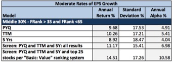
How about that!

Lao Tzu and Aristotle were right. There’s something to be said for growth investing that avoids extremes and focuses on moderation. It’s not macho growth (sky-high growth rates). But it does seem logically aligned with a good probability of the sort of DDM type growth we need.

Wait a minute. Table 4 worked with EPS. What about Sales? Table 5 shows what happens when we re-cast all those screens in terms of Sales Growth.

Table 5

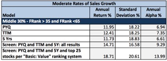
Yay! Sales growth works. Actually, Sales growth works better than EPS growth. This is what we logically expected to see before we went astray with all those single-factor low-DDM-credibility screens.

This is an example, a graduate-level example, of why I keep preaching DDM. Notice that reference to the DDM and the logic of the proxies we need to create got us to a good place we might never have otherwise reached

Valuation Ratios: Q vs. TTM

In connection with the growth discussion, I explained why the PQ consecutive-quarter comparison was inappropriate (and usable only as an indication of noise/momentum). A related issue is use of quarterly numbers as part of a valuation.

I see this a lot on Portfolio123: Pr2SalesQ, EV/EITDAQ, Pr2FrCashFlQ, etc. including Ind variations on all of these ratios. They are not legitimate valuation measures because, as discussed above, we think in annual terms and because seasonality, subtle as well as blatant, precludes us from multiplying by four to convert a Q figure to an annual figure.

Having pre-set ratios along these lines in the database is an unfortunate error that reflects the history of the database. This ratio and other pre-set ones we had before we switched to Compustat (and which we recreated in Compustat) trace back to a now-defunct company called Market Guide, which was acquired by Multex in 2000 and absorbed into Reuters and eventually Thomson Reuters through subsequent M&A and sets of corporate priorities that had little to do with investors making money and more to do with demoing to prospective licensees all the different and cool kinds of things one could concoct if one were to be wise enough to buy a data license.

So you should not presume each and every item among the pre-set ratios is worthy of use. These Q valuation metrics (and others such as ROE computed on quarterly earnings) got there for all the wrong reasons.

Can they ever be use as an indicator of potential future equity performance? Maybe. Remember, it’s not just about value. It’s also about noise and momentum. If enough people trading enough money think the numbers are useful, the stocks can and will behave accordingly. But, it’s not Value. It’s momentum and will succeed or not based on factors relating to noise and momentum. (It’s not for nothing that I’ve seen SA models authored by designers who I know favor Q-based valuation metrics that often have high SA Momentum style scores and, often, low Value scores.) 

If you understand and wish to use these ratios as components of a noise or momentum strategy, go for it. If you are using any of these in order to gauge Value, it’s important that you cease doing so and revise your models, even if they backtest well. To illustrate, let’s look more closely at Pr2SalesQ, a very popular item in Portfolio123.

Case Study: Pr2SalesQ

As previously discussed, investors value stocks on the basis of annual information rather than quarterly information. I’ll acknowledge it’s hard to come up with much outside authority to cite in support of this proposition because frankly, this sort of thing is well understood; it doesn’t typically come up among knowledgeable sources as a topic that needs to be researched or addressed.

Nevertheless, I have come up with some respectable authority, not specifically on Q versus TTM but on something much more fundamental; how we use numbers (the past and hence, not dispositive of investment outcomes) to support reasonable assumptions about the future (that which we actually care about).

One very obvious problem with valuation based on quarterly fundamentals is seasonality, as previously discussed. But that, actually, is the lesser consideration. The primary basis relates to the concept of fundamental condition, or as Graham & Dodd described it, earnings power:

IN THE LAST SIX CHAPTERS our attention was devoted to a critical examination of the income account for the purpose of arriving at a fair and informing statement of the results for the period covered. The second main question confronting the analyst is concerned with the utility of this past record as an indicator of future earnings.This is at once the most important and the least satisfactory aspect of security analysis. It is the most important because the sole practical value of our laborious study of the past lies in the clue it may offer to the future; it is the least satisfactory because this clue is never thoroughly reliable and it frequently turns out to be quite valueless.

Graham, Benjamin; Dodd, David (2008-09-04). Security Analysis: Sixth Edition, Foreword by Warren Buffett(Security Analysis Prior Editions) (Kindle Locations 8886-8891). McGraw-Hill Education. Kindle Edition. (Emphasis supplied.)

Notice what was said in the emphasized text. We use data for one purpose and one purpose only; “the clue it may offer to the future.” We’re not necessarily reproducing what was in the 10-k and 10-q documents (Graham and Dodd devote considerable ink to this idea). And we are not necessarily looking for a fresh or recent view of the company’s performance. If the freshest information provides a clue for the future, then we can use it. If not, we should ignore it. This is the mindset that should guide any strategy that is designed for the purpose of achieving good live (out of sample) performance. Now, let’s continue with Graham and Dodd.

The concept of earning powerhas a definite and important place in investment theory. It combines a statement of actual earnings, shown over a period of years, with a reasonable expectation that these will be approximated in the future, unless extraordinary conditions supervene. The record must cover a number of years, first because a continued or repeated performance is always more impressive than a single occurrence and secondly because the average of a fairly long period will tend to absorb and equalize the distorting influences of the business cycle.

Id at Kindle Locations 8894-8897 (Emphasis in original)

This set of ideas, the quest for a measure of earning power that transcends individual and potentially non-representative occurrences, is what inspired creation of the Shiller P/E:

The price-earnings ratio is a measure of how expensive the market is relative to an objective measure of the ability of corporations to earn profits. I use the ten-year average of real earnings for the denominator, along lines proposed by Benjamin Graham and David Dodd in 1934. The ten-year average smoothes out such events as the temporary burst of earnings during World War I, the temporary decline in earnings during World War II, and the frequent boosts and declines that we see due to the business cycle.

Robert J. Shiller. Irrational Exuberance(Kindle Locations 266-268). Kindle Edition.

Consider what these authorities are saying. They seek to stretch the measurement period in order to diminish the impact of unusual and presumably unsustainable factors that detract from our ability to use historical data to support assumptions about the future.

This is a critical point. We don’t use data because it’s accurate. We don’t use data because it’s good. We don’t used data because it’s proven it has usefulness in the past. We don’t use data because we can justify its relevance to understanding the company’s most recent performance. None of those considerations matter. There is one, and only one, thing that counts: Does the data give us a reasonable basis for making plausible assumptions about the unknowable future? If the answer is “no,” the data should be discarded.

A quarterly PS figure is too tenuous to give us a reasonable basis for making plausible assumptions about the unknowable future. One might argue the same about a single TTM figure. Perhaps this may inspire you to create your own longer-term average. But one thing is beyond dispute. If it’s live rather than backtested performance you seek and you feel unable to cope with the challenges of creating a Shiller-like PS, then a 12-month sales figure is the correct figure to use (a real one and not one that is artificially created from Q*4), and that is so even though Q elevates the “freshest” information.

Admittedly, use of multi-period averages is not necessarily a panacea and poses practical difficulties. But to shorten the frame more than necessary, from 12 months to three, a period inconsistent not just with the seasonal tendencies but with the annual rhythms that characterize the way many companies and customers conduct their affairs and the one most prone to aberrant factors (the timing of orders, manufacturing issues, etc.) is indefensible assuming one is, indeed, looking to data for the clues it offers about the future. We should conserve our energy and defend our use of TTM in lieu of a harder-to-implement 10-year inflation adjusted sales-per-share average.

Consider, too, James O’Shaughnessy, author of the well-regarded but unfortunately titled What Works on Wall Streetand one who certainly cannot be accused of failure to understand factor analysis. He was presumably, quite capable of studying quarterly PS ratios. But he did not do so. He hardly even saw fit to make an issue of the distinction between three- and 12-month sales figures other than the following backhanded reference as part of making a different point:

A stock’s PSR is similar to its price-to-earnings ratio, but it measures the price of the company against annualsales instead of earnings.

O’Shaughnessy at Kindle Location 2542 (Emphasis supplied). See also Richard Tortoriello Quantitative Strategies for Achieving Alpha(McGraw-Hill Finance & Investing, 2008) (Chapter 13) Note that he uses the abbreviation PSR when referring to Price-to-Sales ratios.
.

It’s not that O’Shaughnessy studied PS on the basis of annual versus quarterly data and came out in favor of annual. He didn’t even bother to study the quarterly version of the ratio! I submit his inattention to quarterly PS was due to the fact that “there is no sound theoretical, economic, or intuitive, common sense reason” (What Works on Wall Streetat Kindle Locations 1254-1255) for its consideration. More specifically, O’Shaughnessy states that “if there is no sound theoretical, economic, or intuitive, common sense reason for the relationship, it’s most likely a chance occurrence.” (Id.)

Let’s switch gears now. Having established that use of Pr2SalesQ is not sound fundamentally, let’s consider whether it “works” – really.

I started by creating two single-factor ranking systems:

• PS – Q
  • Pr2SalesQ – sorted relative to universe, lower is better

 

• PS – T
  • Pr2SalesTTM – sorted relative to universe, lower is better

 

Next, I’ll run a series of top-50% and bottom-50% screens using these ranking systems, the PRussell3000 Universe, and a 1/2/99 through 6/16/16 time frame. I used a 4-week rebalancing interval, and also, the 1-week interval favored, it seems to me, by many who use the Q valuation ratios.

What you’ll see in Table 6 is that Pr2SalesQ and Pr2SalesTTM both work. In fact, there seems to be little variation – the identical figures for the annualized returns of the best groups under the 1-week rebalancing protocol is not a typo.

We should not be surprised. The Q figure is part of the TTM. In cases where trends persist, we should expect PS ratios under the two versions to correlate very highly.  Think of it this way. Q is a passenger. TTM is the vehicle. You expect the passenger to be carried along by and go together with the vehicle.

So far, it seems like I’m actually arguing for the Q version. Perhaps the freshest view of the car is best and, assuming trends persist, that is provided by the Q version. But the world can be an unpredictable place. Things happen. And these things are what can make or break you in the market.

As you peruse Table 6, notice in the bottom sections of the table when I specifically set out to measure whether or not Q is, indeed, sitting in the car or whether Q has, for some reason or another been kicked out of the car and forced to walk on its own.

Table 6

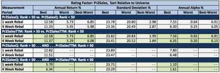
In the third section of Table 6, Q is sitting in the car. The screen was:

• Rating (“PS – Q”) > 50
• Rating (“PS – T”) > 50

Performance here was fine, and very much in line with the separate tests of Q and TTM.

The forth section of the Table is where things get interesting. Now, Q is kicked out of the car and must travel on its own.

• Rating (“PS – Q”) > 50
• Rating (“PS – T”) < 50

Uh oh.

It still works, but it lost a lot of ground when it had to stop riding TTM’s coat tails. This is exactly what the theoretical discussion above should have led us to expect. Valuation is about 12-month measures.

I know many in Portfolio123 try to get around the seasonality issue by doing the valuation sorts based on Industry rather than Universe. Table 7 repeats the tests with all ranking systems set of Industry sorting.

Table 7

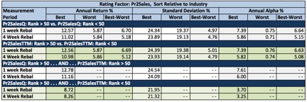
There’s little change in the first three sections of the Table. And we do see some improvement in the fourth, the area in which the Q ratios are out of the vehicle and walking along the side of the road. So we have taken some seasonality out of the picture (to the extent the GICS categories line up with the real world, a process that’s pretty good but which can never be perfect). But remember, it’s not just about seasonality. It’s also, perhaps more, about the need to aim for the longest measurement period we can feasibly get, or at least the need to refrain from shortening it more than necessary.

Even though the Q-Industry measurement is better than Q-Universe, why bother using even the former? What’s the point? It’s wrong fundamentally. And it doesn’t work empirically when the question is properly framed (i.e. it’s not even good data mining).

In sum, if you are going to use a Q-based valuation metric, make sure it’s in the sort of context you’d use with a sentiment factor such as upgrades, or a momentum factor such as a trend indicator or a gap up, that sort of thing. Q items are relevant to momentum and/or noise. But as a value factor, no, absolutely not.