Factor Inversion: When Up Is Down, Good Is Bad, Dumb Is Smart, and Right Is Wrong

2018 has been a tough year in the stock market for many investors for various reasons, but here’s one that gets no play in the financial media at large, comes up blank (in terms of investment-related results) in a Google search, and threatens to shatter the confidence of many seasoned veterans. It’s something not-so-lovingly referred to as“factor inversion” and it’s behind many statements like “such-and-such approach has proven itself over the long term but is cold right now,” and familiar rhetoric to the effect that “even the soundest approaches can’t be expected to succeed all the time, but rather must be evaluated based on the big picture.” There is presently no reliable replicable cure for factor inversion. The first step in getting to a cure, or at least softening the impact, is recognizing that factor inversion is a normal market characteristic for which one must develop strategies to address the effects (one strategy is presented herein).

(Click here for a PDF version of this report.)

Factors and Inversion Defined

A factor, in this case, a stock factor, is a presently-observable attribute that is associated with future share returns. The Price/Earnings (P/E) ratio is an example of a factor. Stocks with lowP/Es are widely expected to outperform shares with high P/E ratios. 

Factor inversion is present when a factor operates in a manner that is the opposite of what should be anticipated. When shares with high P/E ratios outperform lower P/E stocks, the P/E factor is said to be inverted. 

When it comes to stock selection, there are two elements to a inversion:

1. A reasonable expectation that a factor will influence future share returns a certain way; and
2. Real-world outcomes that are the opposite of what we reasonably anticipated.

(Clifford Asness, cofounder of AQR Capital Management, satirically portrayed the inversion phenomenon in his 10/22/18 article on “The George Costanza Portfolio.”)

Identifying Factors

This challenge can be addressed many ways.

Since most share price movements are influenced by general stock-market conditions, the stock market itself (more specifically, the expected return of the equity market) is widely considered to be a factor, and in some quarters (those who believe markets are efficient), the only genuine factor. Most market participants today go further and also consider such things as company size, valuation, company quality, and company investment to be factors. See, for example, the pioneering three-factor schema (consisting of the market, size, and value) proposed in 1993 by Eugene Fama and Kenneth French, their 2015 five-factor expansion (that added profitability and investment), a 2018 critique by David Blitz et. al. chiding them for having failed to include Momentum and Volatility, and if this isn’t enough, research by Guanho Feng, et. al., Jason Hsu, et. al., Soosung Hwang, et. al addressing the proliferation of new factors that now collectively comprise the “Factor Zoo” in order to discern more examples of factors.

What about dividend yield? Is that a factor? Many see this as an attribute of a desirable stock. However researchers argue that it’s not a factor since empirical research demonstrates no relationship between higher dividend yields and greater future share returns. The way Fama and French put it, the increased return from the dividend yield tends to be offset by declining share prices. Critics of yield are correct; higher yield is not associated with expected superior returns, but their research is still wrong.

While they did not err in a computational or statistical sense, their research was simply pointless. Market practitioners know that higher yields exist because share prices are bid down (relative to the level of dividends) due to investor fears that the dividend will be reduced or eliminated (typically due to expected poor company performance). Given this cause and effect, it was never rational to hypothesize an association between high yields and superior future returns. In fact, the more reasonable topic for research is whether lower yield (down to and including zero) is the factor to be positively associated with future equity returns. (Low- and zero-yield companies tend to reinvest profits aiming at internally generated growth.) The error in the yield factor research occurred simply by having undertaken the project. Had empirical study supported the high-yield hypothesis, one would have no choice but to expect computation error, or lucky coincidence.

For convenience, factor investors and researchers tend to speak of factors with reference to a relevant  investment style. Hence P/E would be considered a value factor. Other value factors would include price/book, price/sales, price/free cash flow, etc. 

Researchers usually define factor with reference to a single idea. For example, Fama and French defined their value factor as Book Value-to-Market, the ratio of a company’s book value to its market capitalization (many practitioners today express the same idea in terms of per-share Price-to-Book (P/B). I think this approach is problematic because it increases the probability that the factor will misrepresent the influence of the attribute. If, for example, a company is losing money or is experiencing a temporary surge in earnings due to a gain on the sale of an asset, P/E (assuming that is the ratio being used to define the factor) would be affected in an inconsistent and non-representative way. Similarly, if a company just made an acquisition that will lead to a big jump in sales going forward, the P/S (which is based on the latest reported figures) would look unrealistically high due to use of an unsustainably small sales tally in the computation. 

Hence utilizing single data items that are so easily altered by standard (albeit erratically occurring) business transactions to represent entire factors can be a misleading and risky strategy. I prefer to define a factor as a collection of items (i.e. a portfolio of items). For example, Value is not just defined as P/E or a Price/Book ratio. I define it through six ratios: (1) P/E with earnings based on the last flour reported quarters; (2) P/E with earnings based on the estimate of EPS for the current fiscal year; (3) the P/E to expected growth ratio (PEG); (4) Price/Sales; (5) Price/Free Cash Flow; and (6) Price/Book. Statistically, these six items are likely to be highly correlated with one another when assessed over a large sample. As a result, quants may reject this approach. However, my approach is defensible, as I’m looking for a comprehensive expression of value that is truly relevant to the assessment of an individual stock. Just as the investor uses stock diversification to reduce idiosyncratic risks from a single stock, I use item diversification to reduce idiosyncratic risks from a single item. 

My Factor Collection

It’s tempting to use statistical study to identify relevant factors (i.e. item collections). But such “curve fitting” exercises (where we hunt for trends that describe historic relationships between attributes and equity returns) are dangerous in that they do not tell us whether the relationships we observe are rational or coincidental. I instead rely entirely on financial theory to tell me what factors to consider. Starting with the foundational truth that the fair price of a stock is the present value of future cash flows the shareholder expects to receive, progressing through such well established mathematical formulations as the Dividend Discount Model and the Capital Asset Pricing Model, and adapting those ideal formulations to the prediction challenges that bedevil us in the real world, I work my way down to the following framework: 

P/E = 1/(R-G), where

• P = Price
• E = Earnings
• G = Expected future growth
• R = Required Rate of Return, which is

R = RF + (ERP * B), where

• • • • • • RF = Risk-Free Rate of Return
          • ERP = Equity Risk Premium
          • B = Beta, a measure of company specific risk

(For more detail on the logic behind this, click here for a Strategy Design Cheat Sheet I created to show Portfolio123 users how to use financial logic to develop rules-based stock-selection strategies.)

Market items RF and ERP address asset allocation choices, not stock selection. The latter uses P, E, G and B (the only company-specific item used to compute R). We can re-phrase B in terms of its fundamental source, Q (Quality). Therefore, the goal is to identify and invest in companies for which P/E is not necessarily low, but low relative to G and/or Q. Each of these would, upon rising, exert upward pressure on P/E and vice versa. 

Here, then, are the five factors (collections of items) with which I work:

• Value: This is the most obvious choice, the factor that’s probably used by everybody. It assumes that all else being equal, shares priced lower relative to some measure of shareholder wealth are preferable.

• Quality: This refers to such well-known items as margin, turnover, financial strength, and return on invested capital. These are the fundamental drivers of future sales risk (volatility), future earnings risk, future share volatility, and finally, future Beta. I presume higher Quality is associated with probably lower future Beta. As a result, my use of the factor presumes that all else being equal, higher Quality (lower business risk) makes stocks more desirable (supports a higher P/E) than lower Quality. 

• Growth: Consistent with what investors would logically assume, higher Growth is preferable to lower Growth. But this factor, based as it is on data from the past which can’t be assured to have predictive value, is limited. Therefore, I view articulation of the growth factor as more an art than a science. Put another way, I approach growth as if I were a police detective searching among visible clues to the identity of an unseen perpetrator. I use Growth (historical), Momentum, and Sentiment (behavior of Wall Street analysts) as potential clues (proxies) that can help me infer the existence of an event for which there are no eye-witnesses (future growth).

• Momentum: This refers to share-price momentum and is one of two proxy factors I consider to shed light on investment community expectations of future growth. (Note that I define Momentum broadly to include the entire field of Technical Analysis.) This is an important justification for any use of trend-based Momentum by anybody. Suggesting that Stock XYZ outperformed in Period 2 because it showed strong momentum in Period 1 is preposterous. It is, however, very sensible to assume that XYZ outperformed in Period 1 because of the market’s response to Situation A (a new product, enhanced company efficiency, market share gains, etc.) and that because Situation A persisted into Period 2, the stock continued to outperform. Hence use of trend-based Momentum as a factor (higher is better) is tantamount to a bet on persistence (of whatever was driving the stock in the past). On the other hand, Momentum based on oscillation indicators are based on human tendencies to over-react and correct.)In terms of my logical framework, strong Momentum is the functional equivalent of positive investment community expectations regarding future company prospects; i.e., Growth.

• Sentiment: This is the other proxy factor that stands in for Growth. It utilizes such items as analyst estimate revision, analyst recommendations and earnings surprise. Higher scores in my sentiment factor are presumably consistent with better expectations of future growth and hence are preferable for stock selection. This factor makes a unique contribution to the mix in that it incorporates presumably informed human judgement, which from time to time raises issues of trustworthiness, but is still important given our task of looking to future growth, an endeavor that can never be fully quantitative. 

Working, as I do, on Portfolio123, I express each of these factors as a ranking system through which I score individual stocks (and favor those with higher ranks). For real-world stock selection, I can use a ranking system as part of a screen that narrow a broad universe to a manageable number of potentially interesting candidates (e.g. a rule limiting consideration only to companies with Quality ranks above 90 on a worst-to-best scale of zero to 100) and/or as a basis for sorting the list of candidates in order to identify a manageable number of final selections (e.g. sort the 250 potential candidates using the Quality ranking system and select the best 20). For details of these five ranking systems, click here.

Studying Factor Performance – Method

This study represents another way to use a ranking system. By examining historical performance of a variety of ranking systems (i.e. how the best ranked stocks performed, how the second best group performed and so on down to the worst group), I’ll be able to easily see and measure inversions, how often they occur, how regularly or irregularly they occur, and how severe they have been.

Therefore, for this study, I used the Ranking System performance capabilities of Portfolio123 to measure the performance of each ranking system for each calendar year from 1999 through 2017 and year-to-date 2018 (through 10/28/18). The ranks are calculated against a universe that approximates the Russell 3000 and from which stocks priced below 3 are omitted.

The stocks are sorted from best to worst and divided into five quintiles, or “buckets” and the performance of each bucket is tabulated. The buckets are labeled such that this highest numbered bucket, 5 in this study, is the one that will, if the factor performs as expected, produce the highest level of performance. (Note: For some ratios, such as Value, lower ratios are preferable. The sorting and scoring protocols are such that the best values, the lowest ratios, will produce higher rank scores, thus maintaining consistency across all items.)

Figure 1 is an example of the Portfolio123 output produced from such a test. The colored bars provide a quick visual summary. However, numerical values for each bar are reproduced at the bottom of the Figure. These numerical values are the ones recorded in the study.

Figure 1

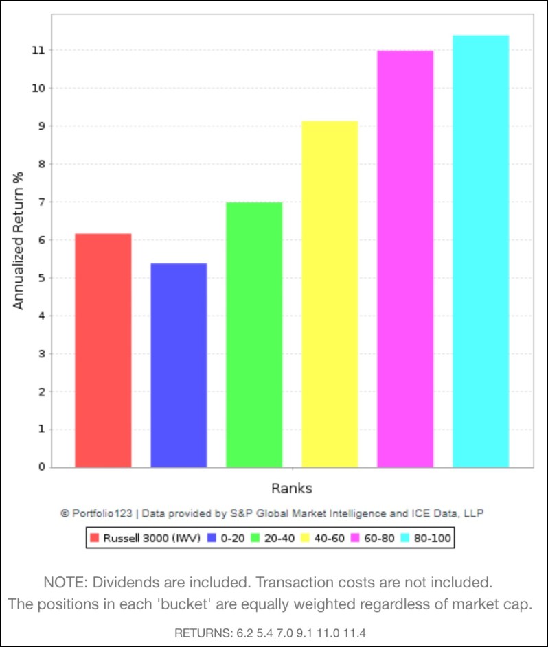
This study focuses primarily on the difference between Bucket 5 (rank scores 80-100) and Bucket 1 (rank scores 0-20). There are labeled in the presentations below as “Best – Worst.”

Detailed Tables for each period for each ranking system show the returns of each bucket, the “Best – Worst” differences, as well as “Best – Mid” (Bucket 5 minus the average of Buckers 2, 3 and 4) and “Mid – Worst” (the average of Buckets 2, 3 and 4 – Bucket 1). These can be seen by clicking here.

The discussion of result below will focus on trends in “Best – Worst.” Factor inversion is present when “Best – Worst” is negative.

Results and Observations

Figures 2 through 6 chart trends in “Best – Worst” for each of the five factors (ranking systems) discussed above. 

Figure 2: Growth 

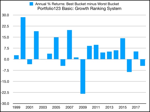
(Note: The Best – Worst difference in 2003 was barely distinguishable from 0.0.)

We see here that Growth is okay, but it may be more trouble than its worth.

Figure 2 looks impressive at first glance, with lots of bars reaching high upward levels. But note the scale on the left. It’s not that high relative to other styles. And it is quite up and down over time. So, too is value, but at least with value, you’re standing on strong theoretical grounds. With growth, you are stuck explaining away your implicit assumption that past performance is predictive of future outcomes. Doing so is not impossible: One can make the reasonable argument that growth is often evolutionary rather than revolutionary, so sudden breaks with history are not likely. That is logical, but much of the empirical success of value stems from the opposite, the tendency of the market to punish investors who naively assume past is future and therefore pay up for high-ratio stocks.

Figure 3: Momentum

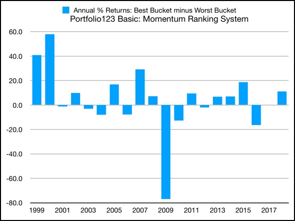
(NOTE: The Best – Worst difference in 2016 was barely distinguishable from 0.0.)

Momentum can produce great returns, but if you’re not nimble, they can quickly turn to ulcers.

At times (such as the present), it’s easy for Momentum investors to do their fair share of chest pounding. But they’d better get it over with quickly because momentum is the least stable factor. Looking at Figure 3, at the times when Momentum was at is best (1999, 2000, 2007, part of 2008, and 2014) in retrospect, those were terrible times to be all in on such stocks, especially aggressive stocks and high-valuation stocks (we’ll see below in Table 1 that momentum and value are negatively correlated).

Figure 4: Quality

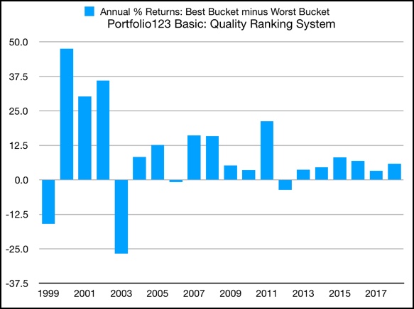
Quality may be the unsung hero in this factor collection.

Except to the extent investors make the connections between such rhetoric as Warren Buffett’s words on inevitability (being able to predict business viability far into the future) or Morningstar’s discussion of moats and Quality, this factor gets little play in market discussion. (We don’t usually see a stock that soars because the latest trailing 12 month return on equity came in ahead of expectations.) In fact, however, Figure  4 shows that Quality has been giving a fairly good account of itself. While positive returns here can be relatively modest, it has lately been less susceptible to out-and-out inversion than the others. 

Quality also illustrates why, in Table 2 below, I present a separate section of summary statistics starting in 2005. Factor investing was invented far before 2005, but in 2005, access to factor investing went mainstream in response to increased availability of reasonably priced data and tools needed to put it into effect. The rhetoric of Quality has been there for ages. New, however, is the ability to express Quality in numerical terms and to do so in a wide variety of creative ways (especially compared to singular definition, “operating profitability” or operating profit divided by book value) offered by factor pioneers Fama and French), which may have helped the market treat differences between high and low quality more rationally than in the past. The well-known Piotroski F-Score, dating from 2000, was an early example of a more comprehensive approach to the topic, and although it was out there during the big 2003 inversion, it’s reasonable to assume quality sensitive investors hadn’t yet fully worked out the kinks in their respective approaches.

Since 2005, Quality has been a respectable performer and a consistency leader. With evolution ongoing and the market likely to become more risky going forward as the multi-generational 1982-2015 plunge in interest rates fades into history, Quality may gain further prominence going forward.

Figure 5: Sentiment

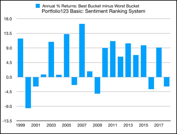
Sentiment has had two lives during the sample period and despite an ongoing inversion, has been better in the more recent period.

In the 11 year period from 1999 through 2009, Sentiment produced four years of strong returns, but  they did not occur in consecutive years. Sprinkled into that interval, we see three years of positive but pedestrian returns, and four separate inversions. After 2009, the picture dramatically changes. We see six consecutive years of sound, if unspectacular returns followed by a rough patch consisting of inversions in two of the last three years (including the present year). 

This is the only factor that is dependent on data that does not relate to companies or their shares. The data comes from the work product of a distinct profession; sell-side securities analysts. We must, therefore, assume that developments in the profession will impact the efficacy of the factor separate and apart from its role as a growth proxy in the context of the framework described above. 

From 1999 and into the 2000s, the sell side underwent massive structural change, having evolved from an ethically-challenged era when analysts worked closely with investment bankers (too closely according to regulators) through a sequence of changes that drove a wedge between Wall Street research and investment banking and replaced often-cozy private analyst-company communication with publicly broadcast and archived conference calls. Old firms were swallowed up or vanished. New firms emerged. Personnel turnover was massive. It could be argued, from Figure 5, that turmoil and change within the profession impacted the quality and usefulness of its work product and added to the normal challenges to be expected for a factor like this (difficulties in forecasting during an evolving investment landscape), but that since the 2008 crash, the profession has stabilized. If that’s the case, we might tie the most recent erraticism to the intellectual challenges of getting things right as we transition away from a nearly 40-year falling interest rate regime to a new one in which rates more likely rise, one in which further equity market advances will need to be driven by earnings rather than rising valuations, and one in which globalization yields to nationalism

Figure 6: Value

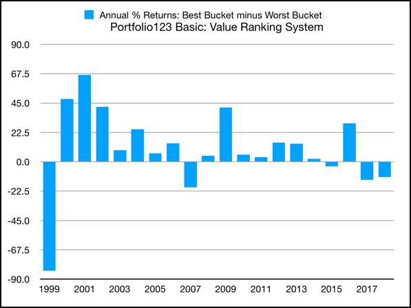
Value is very inverted right now and may come in for some reassessment in the future. If you’re frustrated that your value investing style isn’t working, and is likely keeping you well below benchmarks and competing approaches, take heart: It isn’t you. Figure 6 confirms that it’s the market. 

If you’ve been telling yourself and/or clients to be patient because value, although cold now, works over the long term, take heart: You’re telling the truth.  Table 2 below confirms that value has delivered the most separation between best and worst stocks over the entire sample. Since 2005, it’s been edged out a bit by Quality, which need not be the end of the world since many Value investors are also sensitive to Quality (Table 1 below shows the Value-Quality correlation to be the second highest in the group.)

We also see two other challenges to use of Value. Table 2 shows that Value can be erratic; the ratio of standard deviation to average is second highest, behind only Momentum. But value investors can take comfort in one thing. Prior periods in which the factor was inverted came shortly before some horrific market ugliness. The turn took time to unfold. But when it came, being opposed to value was a terrible stance to have had. Will history repeat? We’ll see.

One thing that bears watching is the persistence of economic trends. Value “works” when investors are punished for naively assuming the past will persist indefinitely. Low-ratio stocks outperform, not because the ratios are low but because fundamentals (usually growth) turn out better than expected on the part of many who naively projected poor past results into the future. Conversely, high-ratio stocks suffer, not because the ratios were high, but because the companies were unable to deliver on the expectations of strong growth (again, in many, cases, based on past performance). Lately, however, with economic trends having persisted for what many would consider a surprisingly long period, there’s been little occasion for ebullient expectations to have gone unfulfilled, and hence little occasion to punish those who pursued too-high ratios. If or when the economy transitions off its notably prolonged trend, there is good reason to expect naive projections to be punished once again and for the value factor to vigorously snap out of its prolonged inversion.

Correlations of the Best-Worst data series’ are presented in Table 1.

Table 1: Best-Worst Differences, Correlations

	Growth	Momentum	Quality	Sentiment	Value
Growth	– –	0.80	0.49	0.33	-0.08
Momentum	0.80	– –	0.29	0.26	-0.37
Quality	0.49	0.29	– –	-0.44	0.57
Sentiment	0.33	0.26	-0.44	– –	-0.64
Value	-0.08	-0.37	0.57	-0.64	– –

Summary statistics for the annual data series’ are shown in Table 2.

Table 2: Best-Worst Differences, Summary Statistics

	Average	Standard Dev	Stan Dev/Avg
ALL YEARS
Growth	5.0	11.4	2.3
Momentum	4.4	26.2	6.0
Quality	9.1	16.6	1.8
Sentiment	4.6	7.3	1.6
Value	9.7	31.1	3.2
FROM 2005
Growth	3.5	11.1	3.2
Momentum	-0.6	25.2	-40.1
Quality	7.3	6.9	0.9
Sentiment	5.7	6.9	1.2
Value	6.2	16.4	2.6

The Reality of Factor Inversion

Even the small sample used here makes it clear that factor inversion is not an aberration. It’s a continually recurring and normal part of the market’s basic fabric.

Sometimes, it’s caused by excess enthusiasm for certain kinds of stocks (see, e.g. 1999-2000). Sometimes, it’s due to a crisis (2008). Sometimes structural change in something that relates to the market (the sell-side-analyst  profession) results in inversions. Sometimes, it’s uncertainty over the direction of the economy or interest rates (as in the present). Sometimes, it’s . . . . It doesn’t matter. It’s always something. And that’s the key to understanding factors and factor inversion.

The stability of factors depends on the stability of the world from which they arise. If the world ceases to evolve and stands still, it would then be possible to cleanly research factors, develop “robust” models, and use them with complete confidence when investing for the future. But the world in which we live has never stood still since the dawn of time, and there’s no reason to expect it to freeze in place in the future. Therefore, there’s no reason to anticipate factor stability. Factor inversion will continue for as long as there is a stock market. Investors must accept that and move forward on that basis.

Investing in the Face of Inevitable Factor Inversion

It’s unrealistic to think we can eliminate factor inversion. It may at times appear we can do so: Data mining (the practice of intensely analyzing historical data with the aim of developing a model that describes behavior in the sample period(s) to a statistically significant degree) can be used to generate studies in which it looks as if we have found a solution. But approaches suggested by such exercises should not be used in real time with real money. Studies like these rely on the past and involve interpolation (describing characteristics of a known and defined population). Investors, however, depend on the unknown and unknowable future and must, hence aim to extrapolate (use historical study to describe characteristics of a different and unknown population that may or may not resemble the sample). The disjunct between the interpolation associated with data mining and the extrapolation of investment reality is the logical foundation upon which warnings against reliance on past performance stand.

That said, there are steps we can take to mute the impact of factor reversion. The key is to make  plausible assumptions, but refrain from overestimating the precision of our efforts. This fundamental and heuristics approach to factor investing yields superior results to a purely quantitative approach, and is based on the following five principles, all of which can be used to help us cope with the inevitability of factor inverted markets:

1. Don’t naively chase a hot factor expecting strength to persist.

We operate today in a highly informed highly concentrated market (i.e. heavily institutional) in which fewer and fewer decision makers (with computerized decision makers taking on larger roles) move more and more money. When something gets hot, it tends to get very hot (see, e.g. Momentum in the early part of the sample shown in Figure 3). Extremes, when they get corrected as they inevitably do, tend to correct with comparable vigor.

2. When it comes to cold factors, be aware of the mean reversion phenomenon.

As long as a factor bears some reasonable relationship to sound investment theory, we have a right to assume inversions are likely to eventually correct. As this is written, for example, Value is in the throes of a significant and prolonged inversion. While we can’t predict when it will return to form, to assume it won’t — to assume what we now see as inversion is, in fact, the new normal — would require us to articulate a new theory of stock pricing (something that does not flow logically from the notion of a price being the present value of future expected cash flows).

I believe I’m on solid ground when I suggest these two principles break no new ground in the area of factor investing. The next three principles, particularly the fourth and fifth, stray from conventional quantitative factor work.  

3. Recognize that absent an ability to perfectly predict the future, factor inversion will always recur and most likely in unpredictable ways.

This should be apparent from Figures 2 through 6 as well as from practical experience and most importantly, common sense recognition that the world never stands still to the point where we can be sure that past performance can perfectly predict future outcomes. Given this, if one is seeking to support real-world investors, it’s pointless to aim for robust modeling against a very large sample. In an academic sense, the quest for discovery of universal truisms backed by strong t-scores and minimal residual error is tempting. But it must be recognized that such results, when carried forward into the real-world markets,  will encounter factor inversion.

4. Bear in mind that no factor is theoretically sound when viewed in isolation.

A strong factor score for Value cannot be presumed to be associated with prospects for strong equity returns. Any P/E can be deemed attractive or exorbitant based on the relationship between Quality (the stock-specific component of required Return) and expected future Growth.

Reshuffling the core P/E = 1/(R-G) equation, we can make similar assertions about Growth and Quality; G = R – (E/P) and R = (E/P) + G.

If we observe empirical data that suggests a factor is working in isolation, the appropriate response is not to reject the P/E = 1/(R-G) formulation but instead, to use it to interpret market behavior. Value “works” when investor expectations regarding Quality and/or Growth do not pan out. The most recognizable example of this is when high P/E stocks falter because growth expectations turn out to have been too optimistic. Conversely, value does not work (i.e. is inverted) when companies deliver on growth expectations.

In sum, the key to understanding factor inversion lies in the P/E = 1/(R-G) formulation.

This is so, even for factors not expressly articulated here. Consider the so-called small-cap effect, the notion that small capitalization issues are expected to outperform larger issues.

There are two potential ways size impacts the 1/(R-G) expression. The most recognizable impact is through G. Small companies can be presumed to have more opportunities for growth. Empirical observation may support or refute that depending on how and using what samples a study is conducted. The impact of size on R (Quality) is more consistent. Company size translates to economies of scale, or fixed costs being a lesser burden on the income statement. Also, larger companies are more likely to be more diversified, even within a single industry classification (a wider variety of products, customers and so forth. As a result, larger companies are likely to experience less earnings volatility and, by extension, share volatility. Therefore, the “small cap effect’ will be described as valid at times when the market is more tolerant of business risk. And inversion occurs when the market becomes less willing to take on business risk.

5. Consider a holistic approach that accounts for Value, Quality, and Growth (Growth itself and/or the Momentum/Sentiment Growth proxies) 

A multi-factor approach that combines Value, Growth and Quality makes sense because that is the way factors are supposed to work. It won’t prevent inversion. If we refrain from isolating factors and cease relying on artificial notions such as the inherent superiority of low P/E, etc., we’ll at least be better positioned to understand inversions and have the wherewithal to resist compounding a difficult situation by rotating into fleeting winners at the wrong time.

A multi-factor approach is not by any means a silver bullet. There are many potential ways to articulate each factor and some are likely to be more effective than others. This is especially so with Growth and Sentiment/Momentum proxies (in fact, the entire field of Technical Analysis can be considered and aspect of the Momentum factor). Even Quality lends itself to more variety than might be realized at first glance. (Earnings Quality is part of this area.) The repertoire of potential Value expressions is large and generally well known. But there are opportunities to excel though one combines value ratios into a portfolio of ratios and relates Value to the other relevant factors.

The next section will examine a creative holistic approach and see how, although it has not banished factor inversion, has succeeded in making it more explainable and manageable than any of the approaches  illustrated in figures 2 through 6.

Case Study in Holistic Factor Investing: The Chaikin Power Gauge Ranking System

Wall Street veteran Marc Chaikin has long been associated with technical analysis. Several of the indicators he created, such as the Chaikin Oscillator and Chaikin Accumulation/Distribution (Money Flow), are standards in the field. More recently, Chaikin, using Portfolio123, developed his Power Gauge ranking system, which is a holistic multi-factor approach that considers the full range of combined factors discussed above, to study the top factors that he believes drive stock performance. (Disclosure: In my capacity at Portfolio123, I conferred frequently with Chaikin as he developed the model and since August 2018, I have been formally associated with Chaikin Analytics in addition to my ongoing work with Portfolio123.)

Chaikin does not organize and present the Power Gauge in terms of Value, Quality and Growth, as I did above, but all of the elements are present and consistent with the notion of factors as presented in this paper. The specific Power Gauge formulations and weights are proprietary but the general formulation is presented on chaikinanalytics.com as follows:

• Value (Financial Factors)
  • • Long-term debt to Equity
    • Price to Book
    • Return on Equity
    • Price to Sales
    • Free Cash Flow
• Growth (Earnings Factors)
  • • Earnings Growth
    • Earning Surprise
    • Earnings trend
    • Projected Price/Earnings Ratio
    • Earnings Consistency
• Technical (Technical Factors)
  • • Relative Strength vs Market
    • Chaikin Money Flow
    • Price Strength
    • Price Trend ROC
    • Volume Trend
• Sentiment (Expert Factors)
  • • Analyst Estimate Trend
    • Short Interest
    • Insider Activity
    • Analyst Ratings
    • Industry Relative Strength

Obviously, Value is important in this model, but its application is far from naive. No matter how well a stock rates in terms of low value ratios, it cannot be ranked highly unless Quality is sound and unless Growth prospects are favorable. Growth is represented through the basic historic data as well as through the Sentiment and Momentum proxies (with Technical analysis, reliant as it is on price and volume data, being in the Momentum family under the schema I use). The selection of these 20 factors, and their weights, came about through very human consideration of the way they interact to select promising stocks. This is consistent with what Chaikin frequently refers to as “the smell test” and with one of the most important but least-quoted lines from James O’Shaughnessy’s What Works on Wall Street: “If there is no sound theoretical, economic, or intuitive, common sense reason for the relationship, it’s most likely a chance occurrence.” 

What makes the Power Gauge especially interesting as a case study is the way its articulation and treatment of what are, deep down, standard factors, differs from conventional academic factors (each of which is defined in terms of a single item whose efficacy had to be established through statistical testing through the multiple regression technique and/or, perhaps, by a significant-item identification protocol that narrows a large collection of similar items to the one(s) shown to be most statistically appealing during the sample periods.)

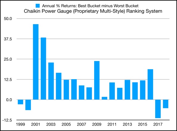
Figure 7, which charts the performance of Power Gauge in the same manner as was done in Figures 2 through 6 for Growth, Momentum, Quality, Sentiment and Value respectively, confirms that even the Power Gauge system is not immune to factor inversion. The question, though, is whether the impact of factor inversion is more tolerable and manageable in Figure 7 than in Figures 2 through 6.

Figure 7

Tables 3 and 4 recreate the Correlations and Summary Statistics shown in Tables 1 and 2, only this time with the Chaikin Power Gauge system included.

Table 3: Best-Worst Differences, Correlations

	Growth	Mom.	Quality	Sent.	Value	Chaikin
Growth	– –	0.80	0.49	0.33	-0.08	-0.24
Mom.	0.80	– –	0.29	0.26	-0.37	-0.39
Quality	0.49	0.29	– –	-0.44	0.57	0.20
Sent.	0.33	0.26	-0.44	– –	-0.64	-0.20
Value	-0.08	-0.37	0.57	-0.64	– –	0.62
Chaikin	-0.24	-0.39	0.20	-0.20	0.62	– –

Table 4: Best-Worst Differences, Summary Statistics

	Average	Standard Dev	Stan Dev/Avg
ALL YEARS
Growth	5.0	11.4	2.3
Momentum	4.4	26.2	6.0
Quality	9.1	16.6	1.8
Sentiment	4.6	7.3	1.6
Value	9.7	31.1	3.2
Chaikin	11.8	14.1	1.2
FROM 2005
Growth	3.5	11.1	3.2
Momentum	-0.6	25.2	-40.1
Quality	7.3	6.9	0.9
Sentiment	5.7	6.9	1.2
Value	6.2	16.4	2.6
Chaikin	8.7	8.9	1.0

I believe the factor inversions experienced by the Power Gauge, while every bit as disheartening as any other kind of market setback, are much more analyzable, manageable and hence tolerable than what we see elsewhere.

The most striking thing about Figure 7 is the way the inversions do not, even at an instantaneous first glance, appear random. They are clustered so we immediately recognize that they should not be deemed a “new normal.” Looking more closely, we see that the inversion clusters have come at times to significant upheaval in the market. 

It’s easy to identify the upheaval that drove the 1999-2000 inversion; the dot-com bubble. Had the Power Gauge been live at the time (the data shown here is produced via backtesting), it would have been easy for anyone with no interest in fundamentals, analysis, and so forth, to have rotated out of highly-ranked Power Gauge stocks into the easily visible and widely discussed runaway winners. But looking back, we know (and found out very quickly) how horrible the financial consequences of such impatience would have been.

Fast forwarding to the present, we are in the throes of another inversion, primarily from Value and also from (historic) Growth and Sentiment. Generally speaking, much of this stems the market upheaval associated with it can be tied to the end of the multi-decade falling-interest rate regime and the emerging shift to a new one characterized by flat rates (at best) or more likely, in my opinion, rising rates. Add in a hefty does of the usual sources of equity-market angst (earnings, trade, politics, global relations, etc.) and there we have it. 

I prefer, however, to not rest here. Every market day since the beginning of markets has been accompanied by similar collections of worry. However, the soundest investment decision was not to sell ownership of productive assets when ancient Mesopotamia started to falter, etc., etc. etc. When seeking to understand a factor inversion, we need to go beyond the usual litanies of bearish arguments and look for that which is unusual or distinct.

Today, the change in interest-rate regime qualifies. But we can go deeper, as I did on October 12, 2018, when I described an unusually strong risk-on Wall Street attitude, which I measured and charted through the relationship of the iShares Edge MSCI USA Momentum Factor ETF (MTUM)  relative to the iShares Edge MSCI Minimum Volatility ETF (USMV). It’s not just a matter of Momentum having outperformed Minimum Volatility. It’s the unusual relative strength exhibited by Momentum, a spike, if you will, that started in late 2016, around the dawn of the Trump era. Combining that with what we know of the impact of Trump on business (the tax cut and the pro-business sentiments now resident at 1600 Pennsylvania Avenue) as well as the steady stream of favorable economic data, I think we have our answer to the present inversion. Why invest in Value (the efficacy of which depends on investors getting punished for exorbitant optimism and rewarded for avoiding the trap of excess pessimism, both camps deriving their respective attitudes by naively extrapolating past earnings trends) when optimistic assumptions continue to be borne out by strong results (meaning high P/E stocks keep on chugging). Compounding the challenge is the difficulty many professionals are experiencing in adapting to the changing regime (i.e., the Sentiment inversion) and changes within the business world in which tomorrow’s winners may differ from those of the past (thus contributing the the Growth inversion).

The recent past hasn’t been the age of fundamentals, of ratios, etc. It’s been the age of “FANG” stocks (Facebook, Amazon, Netflix, Alphabet-Google). 

The Power Gauge is not all Value and it does not ignore expectations and Momentum. However, it pays enough attention to the Value factor that we see the same inversions in the Power Gauge as well. Had Power Gauge been predominantly momentum driven, we would not likely be seeing inversions at present.

So as with 1999-2000, we can ask the question: Is it a good idea to rotate out of favorably ranked Power Gauge stocks and into FANG stocks, FANG-like stocks, and other highly ranked Momentum plays? 

We know that to outperform in todays market we need to rotate into these high momentum stocks, but we need to consider whether doing what it takes to outperform right now is a good idea. Do we really want to sacrifice what we know, over time, are consistent solid returns to go chase the high returns we see now, even though we know we will pay for it later?

Conclusion

Whether to stay with Power Gauge or any other holistic approach that’s been pummeled lately by the inversion (due mainly to value inversion) or rotate into a different approach that have been delivering better performance lately is, of course, an individual choice.

As the new interest-rate business regime settles in, I expect the Growth and Sentiment inversions to correct. The real key is the Value inversion.

Maybe this time it will be different. Maybe this time the economy and earnings will continue to soar in line with rosy expectations. If great expectations, implemented by purchasing high-valuation stocks, continue to be indefinitely rewarded, then the Power Gauge is not likely to satisfy going forward (nor is any other genuinely holistic approach). An end to a value inversion would not require a recession, and actually, the post dot-com inversion ended when the economy came out of recession. It requires an end to satisfaction of exorbitant expectations either way. Shares of highly regarded companies can falter even in good times, if the times are not as spectacular were the assumptions incorporated into high P/Es. Shares of poorly regarded companies can flourish if recession forecasts prove wrong and earnings outperform pessimistic projections.  

It is my view that the economy and market will be fine going forward, but that success will require better  less extreme expectations than those that worked since late 2016. If that’s so, the value inversion will correct as investors once again get punished for paying up in response to extreme historic growth and expectations and get rewarded for recognizing that past sluggishness is likely to mean revert upward. 

Whether you agree or disagree, there is one thing  upon which I believe we can all agree. The use of a holistic multi-factor approach to investing that takes full account of the P/E = 1/(R-G) dynamic allows us to better understand what we’re seeing in the market, articulate more sensible questions, and come up with answers that are more likely to be sustainably consistent with our own goals and risk tolerances.