PDF Version: P123 Strategy Design Topic 3E – Special topics in Valuation
It’s time to finish the topic of valuation. Having covered price to earnings, sales, cash flow and book value, you now have the tools to effectively factor valuation into your models. There are other metrics you can use, for example involving EBIT, EV/EBITDA, or price to other balance sheet measures beyond book value. The concepts, however, don’t change. Start with the DDM as a theoretical foundation and, using the ratios we covered as examples, relate your custom ratio to the task of moving us toward the ideal DDM valuation. Do that by going beyond the basic sorting of ratios and consider, too, the “all else” items that impact whether the ratio operates as one might expect.
Before we leave this topic, let’s look at what may best be referred to as special topics. There are two of these: Asset Plays, and Discounted Cash Flow.

Asset Plays
An asset play is a situation wherein investors, sort of, throw fundamentals out the window and value stocks based on what they believe private buyers would pay either for the company as a whole or for parts of it. With the latter, the goal is to have the parts worth more than the whole: In other words, each of two subsidiaries is assumed to be worth $100 million for a total buyout value of $200 million while the actual market cap for the company as a whole is only $150 million.
Valuing these situations, however, can be a head scratcher, not so much because we don’t know how, in theory, to value businesses (we definitely know how to do this) but because real-world appearances suggest noting along these lines is taking place. When analysts write in detail on the topic, often they act like real estate appraisers; they value based on study of comps, valuation of comparable businesses.
I’ll simplify: In truth, there isn’t a dime’s worth of difference between valuing Wal Mart or valuing a no-earnings asset play. In both cases, it all comes down to the exact same thing: DDM (the Dividend discount Model – and any logical more implementable proxies we might devise).
Don’t draw conclusions from the reality that asset plays are not discussed in such language. One of three things is happening.
- On the one hand, private buyers (and/or investment bankers) may be doing DDM-style valuations on their own for the companies or for individual subsidiaries. Successful buyouts despite premium takeover prices involve situations where the business was, indeed, worth more to the private buyer than to investors in the public market.
- One way this can happen is through our old friend P=V+N, price equals value plus noise. N becomes irrelevant in the private market. And that creates opportunity where N is acting as a depressant in the public markets. (If you work with the noise-value concepts discussed earlier, you’ll see many instances of noise winding up with a negative number.) Therefore, you can try to identify potential buyouts by modeling based on noise that is negative or very modest coupled with fundamentals that suggest the stock deserves better (don’t assume noise should be zero, determine, based on empirical efforts, a benchmark level of noise).
- A private buyer may be assessing the risk component of k (cost of capital) and/or g (growth) differently from what’s being done in the public markets. Sometimes, this is simply a matter of opinion. The Street thinks a company can grow 5% per year. Mr. P (as in Private) Equity thinks it can grow 12% per year. Often, though, this is more than a simple difference in estimates. A private buyer may believe incumbent management is not doing a good job and that new stewardship will enable the company to reach its potential. Poor fundamental performance relative to peers coupled, perhaps, by less noise in the stock relative to peers may be ways you can build models that find such situations.
- Private buyers are flat-out wrong. Either they did an ineffective job of DDM-inspired valuation. Or, they didn’t bother doing it at all (something that happens, sometimes often). From the vantage point of the Street, we file this under “W” for “Who Cares.” The street got taken out at a premium, pats itself on the back, and moves on to other things. But having spent some time managing a junk bond mutual fund, I’m quite familiar with asset plays from the vantage point of the buyer (i.e. what happens after the acquisition closes and the business vanishes from the public equity markets). The result can look very different there. Instances of inattention to DDM or deficient implementation are plentiful and the results often ugly. This, by the way, is why shares of companies that announce themselves as acquirers tend to experience knee-jerk declines. The Street knows how often private buyers get sloppy and when a company in which they hold shares announces and intention join this not-so-desirable club, investors often adopt a guilty-until-proven-innocent stance. As for us, from our perspective as participants in the public markets, we of the take-our-money-and-file-it-under-“W” crowd, modeling is not easy. We can’t spot these situations through fundamentals because they aren’t being driven by fundamentals.Perhaps the best way to model for situations like this is to seek out instances of rising noise unsupported by fundamentals. But even at that, such models may work better as idea generators (identify a group of stocks for follow-up with case by case study) than as automated portfolios. So even if testing suggests little potential for a model built along these lines, you may want to keep it for use as an idera generator. (There’s plenty of benefit you can get on Portfolio123 separate and apart from creating automated portfolios.)
Throughout this, one thing is clear. DDM is still at the heart of everything (recall that I’m not talking about DDM in the literal sense, since the formula is not real-world usable, but as the core that logically links to the various proxies we can and do devise). When we value asset plays, we’re not using any sort of different secret sauce. The sauce is the same. What we’re modeling for is dysfunction in its application; dysfunction on the part of public market assessment, dysfunction on the part of incumbent management that is not realizing the company’s potential, or dysfunction on the part of the private buyer who, after watching us waltz off happily with the premiums we pocketed, embarks on a slow boat to bankruptcy.
Discounted Cash Flow (DCF)
This is the Holy Grail of securities-analysis education. It’s also the most cynical trick an analyst can pull on naïve and unsuspecting clients when they trumpet their wonderful detailed DCF models.
- On the one hand, DCF makes them look good, incredibly diligent. After all, DDM is, an example of discounted cash flow (using, literally, cash flows instead of dividends). If we’re to respect DDM, as we should given its theoretical stature, how much more deserving of respect is model that eschews the back-of-the-envelope simplicity of D, k and g and plunges instead into the multi-year (sometimes 10 or more years) forecasts of company fundamentals.
- On the other hand, in practice, the models are garbage, complete, total and appalling garbage, so much so that I think of DCF as “Discounted Cash Fluff.”
We see every day how hard it is to forecast one quarter ahead. So how seriously should we take the detailed multi-year forecasts that make up the bulk of these DCF models.
What’s worse is the question of how we cope with uncertainty as to holding period. How many years should we forecast for a proper DCF exercise? Three years? Five years? Ten years? Fifty years? Actually, as with plain old DCF, the answer is: infinity. That, of course, is not done since analyst reports are formatted on the basis of the pre-electronic 8.5” by 11” sheets of paper; even in landscape mode, it’s hard to show much beyond 10-15 years, so infinity is out of the question. What has to and does happen is that the last year culminates in what is known as a terminal value which in terms of practicality, is pretty much along the lines of the DDM’s incalculable-in-the-real-world k – g denominator.
So as un-implementable as DDM is, DCF is worse. DDM applies a terminal valuation to something we can see right here and now, a dividend. DCF applies a similar terminal valuation to a measure of cash flow assumed for X number of years into the future that was derived seat of the pants or from many interim assumptions all of which are no less vague and often more vague than the quarterly estimates we can never seem to get right until companies issue final guidance as the quarter approaches its end. And when I say a lot of assumptions, I mean A LOT. A DCF spreadsheet I created in connection with another project required more than 200 inputs!
But wait. It gets worse. Those terminal valuations are not icing on the cake. They are the heart and soul of the DCF valuation. If you ever get you hands on a DCF model, calculate on your own assumed terminal value as a percent of total value. You’ll be shocked at how high it is; rarely if ever below 50% and often much higher.
A Change of Pace
Now that I’ve ranted and possibly riled you to the point where you’re ready to hurl all sorts of obscene invectives at any who publish DCF models, I’m going to switch gears and – hold on here – offer you a DCF model, better still, a DCF model you can use in Portfolio123.
Here’s the catch: It’s not a conventional DCF model but an adaptation designed to rely on as few inputs as possible with most of them being from historical data. We’ll be using what’s known as the Residual Income Model and in effect, valuing stocks on the basis of discounted future residual income. As is necessary for any exercise of this nature, we to will need a terminal value and it too will loom large in our final valuations. But unlike conventional terminal values, ours are built on a solid foundation (the much more forecast-able future residual income item), will not need to go out very far (even three years can be ample) and rather than assuming perpetual growth to infinity, it assumes zero growth after the forecast horizon (thus building in the often craved often extolled margin of safety or cushion for error).
The Residual Income Model (RIM)
RIM, also referred to in the literature as the Edwards-Bell-Ohlson (EBO) valuation technique, starts with the following framework:
Eq.1 V= C + PVEW
Where, V = Value
C = Capital
PVEW = Present Value of Enhancements to Wealth
Although this appears to differ from DDM, it’s actually a close first cousin. Both models work with the present value of future expected shareholder wealth.
- DDM measures wealth that flows directly into the shareholder’s hand, dividends. RIM measures wealth that flows to the corporation, and presumes, as we do with valuation based on earnings, sales or cash flow, that such streams of wealth can, in the workaday world, serve as reasonable proxies for wealth that flows directly to shareholders.
- DDM starts with a base of zero and uses the present value of future expected wealth as 100% of its valuation. RIM works with a known starting point, a base of existing capital and layers the present value of expected additions on top of that.
Moving on, RIM assumes that the measure of starting capital is the company’s Book Value. That means we start with the notion that the value of a stock is its book value per share. Therefore, assuming no impact from Noise, differences between observed Price per share and observed Book Value per share reflect Wall Street’s dollars-and-cents assessment of company activities that enhance or diminish future wealth. The higher the PB ratio, the greater the expectation re: future wealth enhancement (this concept should have a very familiar ring based on our consideration of PB).
So what does it mean when we see stocks that trade apart from this RIM valuation? We can say it’s noise that arises because (i) investors are paying too much or too little for the wealth enhancement or destruction that is likely to occur, and/or (ii) investors misjudging likely wealth creation/destruction.
Moving now, toward an implementable model, we’ll change C in Equation 1 to BY:
Eq. 2 V= BV + PVEW
Where, V = Value
BV = Book Value
PVEW = Present Value of Enhancements to Wealth
PVEW, the good stuff, starts with the basic measure of corporate prowess; ROE, return on equity. But ROE alone does not tell us whether the company is enhancing or destroying wealth. A company whose cost of equity is 6% percent would be creating wealth if it can use that equity to generate an 8% return. On the other a company that pays 12% for equity capital but earns only 10% is destroying wealth. So rather than working with raw ROE, we’ll measure wealth creation in terms of excess, or “abnormal,” ROE.
Eq. 3 AROE= ROE – CE
Where, AROE = Abnormal return on equity
ROE = Return on equity
CE = Cost of Equity
Having brought ROE into a prominent position in our model, let’s refresh ourselves a bit on what we know.
Eq. 4 ROE= NI/BV
Where, NI = Net Income
ROE = Return on equity
BV = Book value (or equity)
Applying some simple rearranging:
Eq. 5 NI= ROE * BV
That was an important detour. Applying the logic of Equation 5, we can say that Residual Income, the portion of net income that enhances wealth, is:
Eq. 6 RI= AROE * BV
Where, RI = Residual Income
AROE = Abnormal Return on equity
BV = Book value (or equity)
Substituting for AORE using its components, we have this:
Eq. 7 RI= (ROE – CE) * BV
Where, RI = Residual Income
ROE = Return on equity
CE = Cost of Equity
BV = Book value (or equity)
Let’s now apply these concepts to our valuation framework; price equals capital plus the present value of wealth-enhancing activities.
Eq. 8 V = C + PVEW
V = BV + PV future RI
V = BV + PV future (ROE-CE)*BV
Stated more formally:

Where, V = Value
BV = Book Value
RI = Residual income
ROE = Return on equity
CE = Cost of Equity
Equation 9 is the residual income model.
Admittedly, at first glance, this may look every bit as intimidating as DDM or DCF. How on earth am I going to estimate ROE for every one of who-knows-how-many years! Here’s the difference: ROE is probably the single most substantial and persistent metric we have in our arsenal. If you want to move on quickly with RIM, you can take my word for this, for now, until we cover it when we get to Quality (the next Topic). If you don’t want to wait, you can check my posting in the parallel on-line seminar I’m doing for Smart Alpha subscribers, wherein I already posted the Quality topic, which you can get, as a PDF, here: https://drive.google.com/open?id=0BxuIkysU9OYuZGsySFdzRDEwNFE
Either way, what’s important to recognize now is that by recasting the expected future flow of corporate wealth in terms of ROE, we’ve completely changed the game. We’ve taken an impractical unwieldy mess and turned it into something very manageable (a reasonable number of clearly identifiable inputs) and credible (a model dominated by the single most persistent measure of company quality we have). Because valuation is future oriented, it can never be anything more than an approximation. But as approximations go, this as good as it’s likely to get.
Undoubtedly, you noticed that the formal statement of RIM still uses infinity. We could handle that with a terminal RI figure that is divided by k – g, the cost of equity minus a presumed (and smaller) infinite growth rate. But as noted above, we’ll use a more conservative alternative: We’ll terminate our series using a zero-growth final-year valuation.
Now that we have the theory nailed down, let’s start implementing.
RIM Inputs from Portfolio123
Before we actually model on Portfolio123, I’m going to present two RIM spreadsheet templates, a simplified version and an expanded version. Assuming you’re building automated portfolios, as most probably do, these spreadsheets will not be part of your work on Portfolio123 so you can skip this section if you wish. I recommend, however, that you build at least one of these sheets and experiment. I can’t imagine a better way to get a deep feel for the process of valuation than by going through such an exercise with individual companies. No matter how much theory or math anybody knows, there’s noting like getting metaphorical dirt under one’s fingernails through study of companies and case-by-case analysis and valuation. That would make a huge difference in how you approach model building. We’re not just using numbers; every data-point in Portfolio123 means something.
Here’s what we need to work with the RIM spreadsheets I’ll present. Note that not all items are needed for each spreadsheet, and we won’t need the entire collection for the Portfolio123 screen.
- Current Stock Price
- Close(0)
- EPS Estimates for current and next fiscal years
- CurFYEPSMean
- NextFYEPSMean
- Estimated Long-Term EPS Growth Rate
- LTGrthMean (If, as many do, you think these are systemically too high, you can deflate them across the board; e.g., LTGrthMean*.8 (making sure you also account for the admittedly remote possibility of a negative projection, perhaps through use of a screening filter. If you really want to be creative, look for ways to deflate them conditionally using the EVAL function).
- Dividend Payout Ratio
- PayRatioTTM
- You can usually use the trailing 12 month ratio as published on Portfolio123. These numbers tend to be tolerably persistent. But aberrations occur, as, for example, when a company newly initiates a dividend or when the trailing 12 month ratio was distorted by temporary factors that inflated or depressed earnings.You can play the probabilities and try to diversify this away, or use screening/buy rules to repel significant oddities.
- You might also experiment with PayRatio5YAvg
- Book Value per share from latest and prior fiscal years
- BVPSA
- BVPSPY
- Terminal Return on Equity
- This is the most challenging input. It’s the ROE we assume the company will generate at some point in the future when competitive and other businesses advantages that presently lead to above- or below-average returns have had time to revert toward the mean. We can use the industry average trailing 12 month ROE as an automated input but this is the item we’d most likely want to revise on our own. The industry trailing 12 month and 5-year average ROEs and the company trailing 12 month and five-year average ROEs can combine to establish a context that can help us formulate a rational assumption, bearing in mind that ROEs are generally persistent over time subject to tendencies of extreme values to gradually revert toward the mean.
- For the Portfolio123 version of RIM, we won’t actually use this. But working with spreadsheets and coming up with assumptions will be an incredible learning experience. If I were Donald Trump, I’d tell you that it’s going to be “amazing.”
- Cost of Equity
- On paper, this input seems horrific, if not impossible. But we live in a world in which we’d rather be vaguely right than precisely wrong. We can handle this in a manner that, if not accurate, should be sufficient to avoid interfering with the ability of other parts of the model to give us investable answers. We touched on this when we discussed Noise-Value and the same kinds of spit-and-chewing gum approximations can be used here too.
- For your reference, here are Google-doc links to a set of four PDFs I previously posted on this topic
The Residual Income Model Spreadsheet – Simplified Version
Figure 1 illustrates the entire spreadsheet.
Figure 1 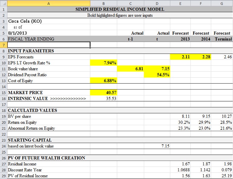
To make sense of Figure 1, let’s work with the basic RIM formulation:
- Value equals capital plus the present value of expected enhancements to wealth.
- That’s in Cell B16, which is the sum of book value (capital) plus Cell E29 plus Cell F29, which are the present values of enhancements to wealth in years one and two, plus Cell G29, which is a the present value of perpetual wealth enhancement beyond year two.
- Enhancement to wealth equals book value (row 19 of columns E, F and G) multiplied by abnormal return on equity (row 21), which is return on equity (row 20) minus the cost of equity (cell B13).
- The book value computations are based on BVt+1= BVt+ Net Incomet– Dividendst
Notice that ROE, the most important component of the formula, is not input. It’s derived from the other data inputs. Consistent with the principles of termination value discussed in connection with the DCF model above, the terminal residual income calculation (cell G29) is based on a static perpetuity, rather than infinite growth.
Table 1 provides the all of the formulas we’ll need.
Table 1
| Cell | Formula |
| G9 | =F9*(1+B10) |
| B16 | =D24+E29+F29+G29 |
| E19 | =D11+(E9*(1-$D$12)) |
| F19 | =E19+(F9*(1-$D$12)) |
| G19 | =F19+(G9*(1-$D$12)) |
| E20 | =E9/((D11+C11)/2) |
| F20 | =F9/((E19+D11)/2) |
| G20 | =G9/((F19+E19)/2) |
| E21 | =E20-$B$13 |
| F21 | =F20-$B$13 |
| G21 | =G20-$B$13 |
| D24 | =D11 |
| E27 | =(D11*E21) |
| F27 | =(E19*F21) |
| G27 | =(F19*G21) |
| E28 | =1+B13 |
| F28 | =(1+B13)^2 |
| G28 | =((1+B13)^2)*B13 |
| E29 | =E27/E28 |
| F29 | =F27/F28 |
| G29 | =G27/G28 |
A version of this model that’s simplified even further (one that uses a single ROE computation for all three forecast years) will be the basis of the RIM strategy we will build below on Portfolio123. But before addressing that, let’s look at an expanded version of the RIM model, one that also requires just eight inputs, including most of the ones seen here, but offers one important avenue for application of analytic judgment – the terminal ROE.
The Residual Income Model Spreadsheet – Expanded Version
Figure 2 illustrates the Expanded version of the Residual Income Model spreadsheet.
Figure 2

The concept is the same as what we saw above; value being the sum of book value plus the present value of future residual income. The differences here are the longer forecast horizon and the introduction of a user-supplied assumption for terminal ROE.
The 12-year forecast horizon used here consists of three phases:
- Two years of forecasts based on explicit EPS estimates, with ROEs and book values being derived based on prior-year book value and that portion of EPS not paid as dividends.
- Five years of forecasts based on EPS assumptions derived from the long-term EPS growth rate assumption. ROEs during this phase continue to be derived based on prior year book value and the retained portion of EPS.
- A five-year convergence period during which the company’s ROE gradually approaches an assumed terminal period (our model assumes a straight-line pattern). During this interval, ROE for each year is a starting point, rather than an end-point to the computations.
- The final year of this period is the terminal value, based on a zero-growth forever assumption.
The terminal ROE is what one regards as the company’s inherent, permanent level of ROE; its inherent long-term capacity to generate returns. For an initial assumption, we should consider using the median ROEs of profitable companies in the same industry. This reflects a general assumption that companies in the same industry should eventually have similar ROEs, after enough time has passed for firm-specific aberrations to fade.
That said, we also have to recognize that industry classifications used by financial data vendors that serve Portfolio123 and other such platforms may not always be perfectly granular. For example, two software companies one of which produces gaming software for consumers and another that produces enterprise-level cyber-security software might both be classified as Software firms yet arguably have different long-term sustainable ROEs even if managerial talent and achievement are the same. On the other hand, it’s easier to argue that two independent energy exploration firms should have the same long-term ROEs. Significant differences observed today, based, for example, on the quality of the properties on which they are drilling, could be expected to eventually diminish assuming hits and misses tend to even out over time.
The level of judgment required regarding terminal ROE is by no means simple. That, however, is not a deficiency in the model. All models require judgments. This particular model focuses most of the judgment on factors that best lend themselves to that which is well within the capabilities of humans: thoughtful consideration of history and the making of analytic assumptions regarding future competitiveness, efficiencies and so forth.
Tables 2 and 3 provide the formulas for this spreadsheet model.
Table 2
| Cell | Formula |
| F16 | =E7*(1+$B10) |
| Copy F16 formula into columns G through J | |
| D17 | =(D18/C8)-1 |
| E17 | =(E18/D18)-1 |
| Copy E17 formula into columns F through O | |
| D18 | =C8+(D7*(1-C9)) |
| E18 | =D18+(E7*(1-$C9)) |
| F18 | =E18+(F16*(1-$C9)) |
| Copy F18 formula into columns F through J | |
| K18 | =J18*(1+K17) |
| Copy K18 formula into columns L through O | |
| D19 | =D7/(AVERAGE(C8,D18)) |
| E19 | =E7/(AVERAGE(D18:E18)) |
| F19 | =F16/(AVERAGE(E18:F18)) |
| Copy F19 formula into columns G through J | |
| K19 | =J19+(($O19-$J19)/4) |
| Copy K19 formula into columns L through N | |
| O19 | =B11 |
| D20 | =D19-$B12 |
| Copy D20 formula into columns E through O | |
Table 3
| Cell | Formula |
| STARTING CAPITAL | |
| C23 | =C8 |
| FUTURE WEALTH CREATION – FORECASTS | |
| D27 | =(C8*D20) |
| E27 | =D18*D20 |
| Copy E27 formula into columns F through N | |
| D28 | =1+$B$12 |
| E28 | =(1+$B$12)^2 |
| F28 | =(1+$B$12)^3 |
| G28 | =(1+$B$12)^4 |
| H28 | =(1+$B$12)^5 |
| I28 | =(1+$B$12)^6 |
| J28 | =(1+$B$12)^7 |
| K28 | =(1+$B$12)^8 |
| L28 | =(1+$B$12)^9 |
| M28 | =(1+$B$12)^10 |
| N28 | =(1+$B$12)^11 |
| D29 | =D27/D28 |
| Copy D29 formula into columns E through N | |
| FUTURE WEALTH CREATION – TERMINAL | |
| O31 | =E18*D20 |
| O32 | =((1+B12)^11)*$B$12 |
| O33 | =O31/O32 |
| RESULTS | |
| O10 | =B13 |
| O11 | =C23+SUM(D29:N29)+O33 |
A Portfolio123 RIM Screen
We’ll start with a screen that calculates values based on a simple version of the RIM model similar to that which was depicted in Figure 8-9.
NOTE: This screen is saved with group visibility here:
https://www.portfolio123.com/app/screen/summary/155018?st=0&mt=1#
- Start by eliminating companies for which the data is likely to be unsuitable for calculating RIM-based valuations.
- We limit consideration to companies with payout ratios between zero and 100 percent.
- We eliminate firms for which book values or EPS estimates are negative.
- Rules:
- PayRatioTTM>=0 and PayRatioTTM<100
- BVPSA>0 and CurFYEPSMean>0 and NextFYEPSMean>0
- Establish a cost of equity. For this particular model, we take a very simple approach. In the interest of simplicity, we’ll use an across the board assumption for all equities. If you want, on your own, you can test sensitivities to varying approaches.
- We define the cost of debt as twice the interest rate on the 10-year U.S. Treasury issue.
- We set the cost of equity as five percentage points above the cost of debt
- Rules:
- ShowVar(@DbtCost,(close(0,#tnx))*2/10)
- ShowVar(@EqCost,(@DbtCost+5)/100)
- Define year-end book values (B).
- Bt is book value per share for the most recently completed fiscal year.
- Bt1is Btplus the product of the year-1 EPS estimate multiplied the retention rate (1 minus the payout ratio)
- Bt2is Btplus the sum or year-1 and year-2 EPS estimates, which is then multiplied the retention rate (1 minus the payout ratio)
- Rules
- ShowVar(@Bt,BVPSA)
- ShowVar(@Bt1,BVPSA+(CurFYEPSMean*(1-(PayRatioTTM/100))))
- ShowVar(@Bt2,BVPSA+((CurFYEPSMean+NextFYEPSMean)*(1-(PayRatioTTM/100))))
- Define ROE as the year-1 EPS estimate divided by the average of Btand Bt1
- Rule
- ShowVar(@roe,CurFYEPSMean/Avg(@Bt,@Bt1))
- Rule
- Calculate the components of the present value of each residual income item.
- v0 is Bt
- v1is abnormal ROE (ROE minus cost of equity) multiplied by Bt with the result divided by the sum of 1 plus cost of equity
- v2is abnormal ROE (ROE minus cost of equity) multiplied by Bt1 with the result divided by the sum of 1 plus cost of equity raised to the second power
- v3 is abnormal ROE (ROE minus cost of equity) multiplied by Bt1 with the result divided by the sum of 1 plus cost of equity raised to the second power all of which is then multiplied by the cost of equity
- Rules
- ShowVar(@v0,@Bt)
- ShowVar(@v1,((@roe-@EqCost)*@Bt)/(1+@EqCost))
- ShowVar(@v2,((@roe-@EqCost)*@Bt1)/((1+@EqCost)^2))
- ShowVar(@v3,((@roe-@EqCost)*@Bt2)/(((1+@EqCost)^2)*@EqCost))
- The RIM valuation, labeled @RIMval, is defined as the sum of v0+ v1+v2+v3
- Rule
- ShowVar(@RIMval,@v0+@v1+@v2+@v3)
- Rule
- Finally, we define @P2RIM, with is the current price divided by the @RIMval.
- Rule
- ShowVar(@P2RIM,close(0)/@RIMval)
- Rule
That’s it, the Holy Grail of our DCF model: @P2RIM, the market price divided by our computation of fair value.
Test Driving the Model
I’m going to use the PRussell3000 universe, the iShares Russell 3000 ETF benchmark, an assumed slippage of 0.25%, 4-week rebalancing, and a MAX testing period (1/2/99 – 12/16/15). For rolling backtests, I’ll assume 4-week holding periods run every consecutive week.
Before we work our way down to investable result sets, let’s get some sense if this has any potential at all to work. I’m going to add rules that select the most favorably valued 20% and then, alternatively, the least favorably valued 20%.
- bullish version (low valuation)
- Frank(“@P2RIM”,#previous)<=20
- Alternative bearish version (high valuation)
- Frank(“@P2RIM”,#previous)>=80
Here are backtest results for each:
Table 4
| Presumed Overvaluation | Benchmark | Presumed Undervaluation | |
| Basic Backtest | |||
| Annualized Return % | 5.65% | 5.15% | 13.59% |
| Stan. Dev. % | 25.42% | 15.82% | 22.72% |
| Max. Drawdown % | -72.70% | -55.77% | -68.07% |
| Sharpe | 0.28 | 0.28 | 0.60 |
| Sortino | 0.39 | 0.37 | 0.82 |
| Beta | 1.38 | – – | 1.24 |
| Annualized Alpha % | 1.00% | – – | 8.34% |
| Rolling Backtest (Excess 4-week Returns) | |||
| Avg. of All Periods | +0.27% | – – | +0.81% |
| Avg. of Up Periods | +1.25% | – – | +3.34% |
| Avg. of Down Periods | -1.28% | – – | -0.14% |
With all the huge approximations we made, we’re clearly onto something.
Pop Quiz:Do you think I missed something important when building the model? The answer will be given later.
Let’s go on and see if we can make this investable. To accomplish that, we need to get the result set down to a reasonable number of stocks: I’ll say 15. I’m going to do that with a Quick Rank based on estimate revision in the past week. I know the screen is pointing me toward good values, so what the heck; I’ll narrow down by going for the 15 stocks the Street might have most likely turned bullish on in the past week.
Here’s the Higher-is-Better sort:
- (CurFYEPSMean-CurFYEPS1WkAgo)/abs(CurFYEPS1WkAgo)
Table 5 shows the test results.
Table 5
| Model | Benchmark | |
| Annualized Return % | +15.85% | 5.15% |
| Stan. Dev. % | 27.79% | 15.82% |
| Max. Drawdown % | -67.55% | -55.77% |
| Sharpe | 0.75% | 0.28 |
| Sortino | 0.88% | 0.37 |
| Beta | 1.32 | – – |
| Annualized Alpha % | 11.40% | – – |
| Avg. of All Periods | +1.34% | – – |
| Avg. of Up Periods | +2.06% | – – |
| Avg. of Down Periods | +0.18% | – – |
Again, we’re on to something. It’s investable. Is it perfect? Down-market performance isn’t great. And we do see some volatility. These are not the sort of numbers a data miner would want to show, but as something that’s clearly theory driven (i.e. we have reason to expect the test results to be representative of what we might see going forward with live money), it’s not the end of the world. Still, the graphic of the trend (Figure 3) shows some late-run volatility that warrants attention.
Figure 3

One explanation comes to mind simply through awareness of what’s been going on in the market; value has not been a hot style lately (as of this writing and toward the latter part of the test period). Let’s test the latest year, not against the iShares Russell 3000 benchmark but against a different one, the S&P 1500 Pure Value Index.
Here are the results:
Figure 5: One-Year Test against Value Benchmark

Table 6: One-Year Test against Value Benchmark
| Model | Benchmark | |
| Annualized Return % | -0.17% | -7.20% |
| Stan. Dev. % | 25.27% | 16.64% |
| Max. Drawdown % | -23.32% | -17.74% |
| Sharpe | 0.12 | -0.32 |
| Sortino | 0.19 | -0.49 |
| Beta | 1.40 | – – |
| Annualized Alpha % | 11.01 | – – |
| Avg. of All Periods | -0.47% | – – |
| Avg. of Up Periods | +3.02% | – – |
| Avg. of Down Periods | -3.31% | – – |
This offers some interesting messages. Frist, we are not necessarily looking at a case in which a once good model went sour. It is a value model and can be expected to suffer during periods in which value goes out of favor. But as a value model, it still generates alpha. We see that it is volatile. While that hurts us in bad times (obviously), we have no shortage of upside volatility during good times. (The lumpy recent trends we saw in Figure 3 don’t indicate a faltering strategy but, rather, some big rallies followed by corrections.) If we want to assume that over the long term, good periods will outnumber bad, well, you know.
Still, it would be nice to get a bit of a handle on the downside. Let’s give it a shot. I’ll add this screening rule:
- Rating(“Basic: Quality”) > 75
The idea here is try to control some of the risk component inherent in value models.
Answer to Earlier Pop Quiz: Did I miss something the first time out? Maybe. Recall that I screened for value and then went right into a sentiment-based quick rank. Wasn’t I supposed to have addressed growth and risk? Actually, I did. Remember, this value model is not a simple ratio. It’s a complex (by Portfolio123 standards) formula in which growth and risk already play huge parts (the LT Growth estimate and ROE both figure prominently, although the latter isn’t addressed directly but is addressed through EPS/BVPS).
So we don’t absolutely have to add anything. But the volatility we see in the tests makes me wonder whether we could stand a bit more in terms of risk measurement. Hence my addition of the Quality ranking system in the context of a screening rule.
Let’s retest (going back to the iShares Russell 3000 benchmark and using the Max period):
Figure 6

Table 7
| Model | Benchmark | |
| Annualized Return % | 16.34% | 5.15% |
| Stan. Dev. % | 23.65% | 15.82% |
| Max. Drawdown % | -67.62% | -55.77% |
| Sharpe | 0.64 | 0.28 |
| Sortino | 0.88 | 0.37 |
| Beta | 1.13 | – – |
| Annualized Alpha % | 10.64% | – – |
| Avg. of All Periods | +1.05% | – – |
| Avg. of Up Periods | +1.40% | – – |
| Avg. of Down Periods | +0.49% | – – |
We definitely made headway in our effort to trim volatility. But since we still see that weakness toward the end of the test period, let’s do another close-up on the latest year.
Figure 7: One-Year Retest against Value Benchmark

Table 8: One-Year Retest against Value Benchmark
| Model | Benchmark | |
| Annualized Return % | -1.42% | -7.20% |
| Stan. Dev. % | 16.56% | 16.64% |
| Max. Drawdown % | -22.38% | -17.74% |
| Sharpe | -0.62 | -0.32 |
| Sortino | -1.16 | -0.49 |
| Beta | 0.89 | – – |
| Annualized Alpha % | -5.42 | – – |
| Avg. of All Periods | +0.88% | – – |
| Avg. of Up Periods | -0.22% | – – |
| Avg. of Down Periods | +1.77% | – – |
We set out to reduce volatility and we did exactly that. The question is whether we went overboard in terms of the return we sacrificed in the recent period. Perhaps, hopefully, there will be less costly ways to manage the volatility, other ways to define the risk test.
Now that you have the model, understand what makes value tick, and have this screen available to you, I’m going to leave it to you to come up with ideas for improving it. Remember, though, if you adapt this to the simulation platform, you’ll have to change ShowVar to SetVar.
Next
We’re done with Value. I don’t mean to suggest there’s nothing more to learn on this topic. There are always new things to learn. That’s the nature of the investing world. But at this point, you know more than enough to work effectively with Value in your strategies. Actually, you probably know a heck of a lot more than many others in the markets right now. More importantly, you now have enough of a theoretical foundation to come up with new ideas of your own.
So it’s time to move on. The next Topic will be one that’s already been introduced and one that hopefully, you now have more interest in than might previously have been the case. It’s Quality.
